Optimal BEM-based Pilot-only Channel Estimation for OTFS
Gianmarco Romano
Università degli Studi della Campania ‘Luigi Vanvitelli’
Francesco A.N. Palmieri
Università degli Studi della Campania ‘Luigi Vanvitelli’
Stefano Buzzi
University of Cassino and Southern Lazio
Giovanni Di Gennaro
Università degli Studi della Campania ‘Luigi Vanvitelli’
Amedeo Buonanno
ENEA
Outline
- Motivation: Develop MMSE-optimal pilot-only channel estimation
- System Model: General multicarrier framework
- BEM Representation: Dimensionality reduction for underspread channels
- Optimal Estimation: Joint channel-symbol estimation via Wirtinger calculus
- Orthogonality Conditions: Zero pilot-payload interference
- OTFS Specialization: Embedded pilot design
- Numerical Results: BER/MSE performance at high mobility
- Conclusions and Outlook
Motivation
- Wireless communications require accurate channel state information for coherent detection and equalization.
- High-mobility scenarios \Rightarrow doubly-dispersive channels with time-varying multipath and Doppler spread.
- Fractional delays and Doppler shifts cause leakage and pilot–data interference across resource elements.
- OTFS modulation has demonstrated superior performance in doubly-dispersive environments, but the fundamental estimation challenges persist across multicarrier systems.
Goal
Develop a unified framework for non-iterative, MMSE-optimal pilot-only channel estimation with explicit pilot design rules, applicable to general multicarrier systems.
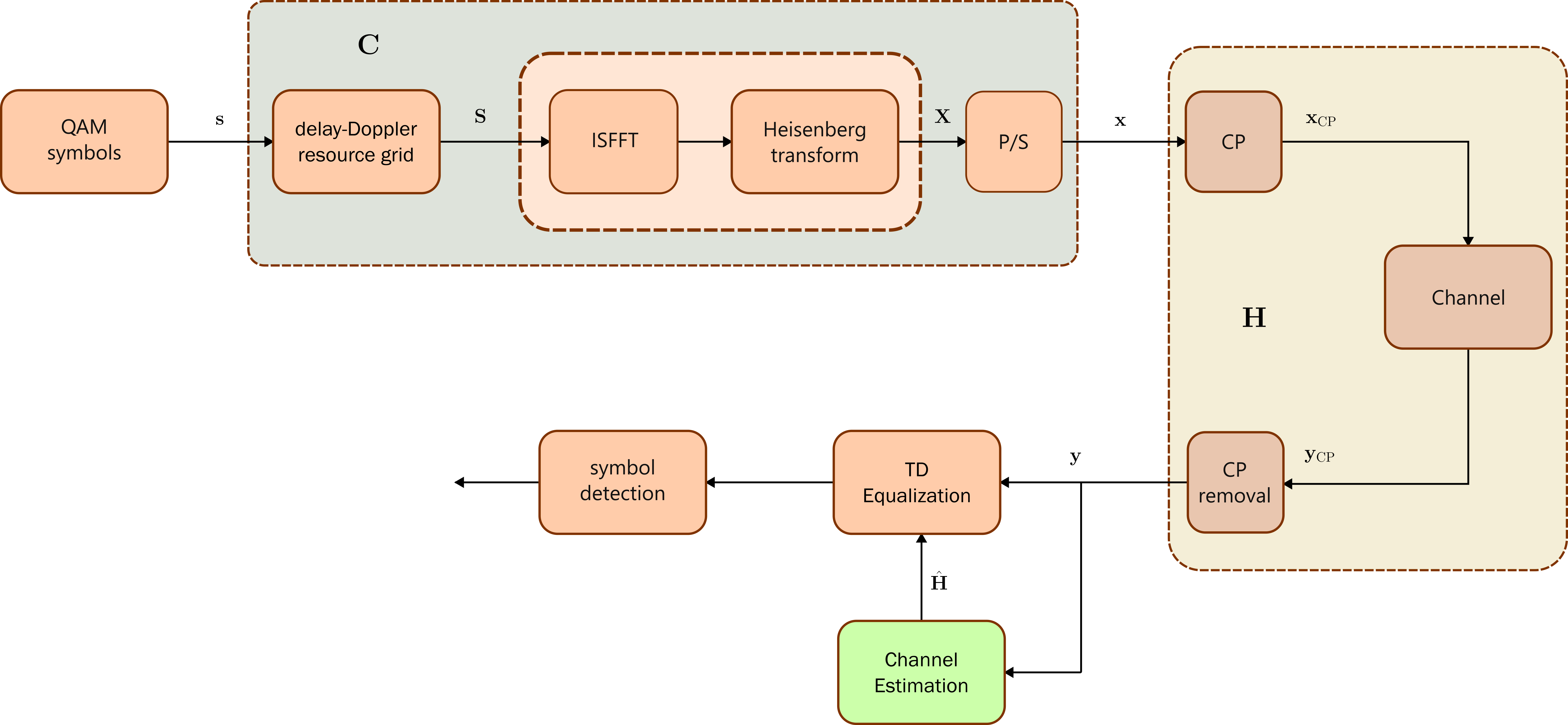
System Model with DD receiver

System Model with TD receiver

System model overview
Block-based transmission of \mathbf{x}\in\mathbb{C}^{N_s} through a time-varying channel h[n,m]
y[n]=\sum_{m=0}^{L-1} h[n,m]\;x[n-m] + w[n].
- L is the channel length (number of taps);
- \mathbf{w}\in\mathbb{C}^{N}\sim\mathcal{CN}(\mathbf{0},\sigma^2\mathbf{I})
- Cyclic prefix (CP) of length N_{\text{cp}} is added to the transmitted block
- Receiver discards CP and channel tail, keeping n=N_{\text{cp}},\ldots,N_{\text{cp}}+N-1.
Unified framework
Coding matrix \mathbf{C}\in\mathbb{C}^{N\times N_s} represents any linear single-carrier and multicarrier modulations (OFDM, OTFS, SC-FDE, etc.)
General system model and assumptions
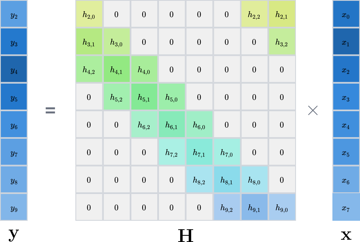
The input–output relationship for the useful block of N samples (after CP removal) can be expressed in matrix form as \mathbf{y} = \mathbf{H} \mathbf{x} + \mathbf{w}, as a linear transformation by the N\times N convolution matrix \mathbf{H} with entries defined by the channel coefficients h[n,m]: [\mathbf{H}]_{m,n} = \begin{cases} h[m+N_{\text{cp}},(m-n)\bmod N], & (m-n)\bmod N \in \{0,\ldots,L-1\},\\ 0, & \text{otherwise}. \end{cases}
Input–output relationship
Delay-tap decomposition
Define the channel coefficient matrix \mathbf{G}\in\mathbb{C}^{N\times L} with \begin{aligned} \mathbf{G}_{n,\ell}&=h[N_{\text{cp}}+n,\ell], \\ &\quad n=0,\ldots,N-1,\ \ell=0,\ldots,L-1, \end{aligned}
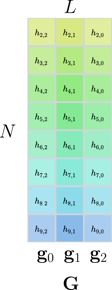
Channel matrix decomposition
\mathbf{H}=\sum_{\ell=0}^{L-1}\operatorname{diag}(\mathbf{g}_\ell)\,\boldsymbol{\Pi}^{\ell},
where \boldsymbol{\Pi} is the N\times N cyclic forward permutation (1-sample circular delay) matrix.
\boldsymbol{\Pi} = \begin{bmatrix} 0 & 0 & \cdots & 0 & 1\\ 1 & 0 & \cdots & 0 & 0\\ 0 & 1 & \ddots & 0 & 0\\ \vdots & \ddots & \ddots & 0 & \vdots\\ 0 & 0 & \cdots & 1 & 0 \end{bmatrix}, \qquad [\boldsymbol{\Pi}]_{m,n}= \begin{cases} 1, & m=(n+1)\bmod N,\\ 0, & \text{otherwise}. \end{cases}
Pilot and payload symbol structure
Symbols \mathbf{s}\in\mathbb{C}^{N_s} are composed of pilots \mathbf{s}_p\in\mathbb{C}^{N_p} and payload \mathbf{s}_u\in\mathbb{C}^{N_u}:
\mathbf{s}=\mathbf{P}_{p}\mathbf{s}_{p}+\mathbf{P}_{u}\mathbf{s}_{u},\qquad N_s=N_p+N_u,\qquad \mathbf{P}_p^T\mathbf{P}_u=\mathbf{0}.
- \mathbf{P}_p,\mathbf{P}_u: (selection/permutation) placement matrices for pilot/payload positions.
- Payload extraction: \mathbf{s}_u=\mathbf{P}_u^{T}\mathbf{s}.
Overall input–output model
Combining modulation with the delay-tap channel model:
\mathbf{y}=\left(\sum_{\ell=0}^{L-1}\operatorname{diag}(\mathbf{g}_\ell)\,\boldsymbol{\Pi}^\ell \mathbf{C}\right)\mathbf{s} + \mathbf{w}.
Receiver-side linear transform (e.g., OTFS demodulation): \mathbf{r}=\mathbf{D}\mathbf{y}=\mathbf{D}\mathbf{H}\mathbf{C}\mathbf{s}+\mathbf{D}\mathbf{w} \triangleq \mathbf{D}\mathbf{H}\mathbf{C}\mathbf{s}+\tilde{\mathbf{w}}, with \tilde{\mathbf{w}}=\mathbf{D}\mathbf{w} (white if \mathbf{D} is unitary).
Vectorized channel representation
The channel matrix \mathbf{H} can be related to \operatorname{vec}(\mathbf{G}) through a symbol-dependent matrix \mathbf{Z}(\mathbf{s}):
\mathbf{r} = \mathbf{D}\mathbf{H}\mathbf{C}\mathbf{s} + \tilde{\mathbf{w}} = \mathbf{D}\,\mathbf{Z}(\mathbf{s})\,\operatorname{vec}(\mathbf{G}) + \tilde{\mathbf{w}},
where \mathbf{Z}(\mathbf{s})\in\mathbb{C}^{N\times NL} is constructed from:
\mathbf{Z}(\mathbf{s}) = \begin{bmatrix} \operatorname{diag}(\boldsymbol{\Pi}^0\mathbf{C}\mathbf{s}) & \operatorname{diag}(\boldsymbol{\Pi}^1\mathbf{C}\mathbf{s}) & \cdots & \operatorname{diag}(\boldsymbol{\Pi}^{L-1}\mathbf{C}\mathbf{s}) \end{bmatrix}.
Key observation: \mathbf{Z}(\mathbf{s}) depends on all symbols \mathbf{s} = \mathbf{P}_p\mathbf{s}_p + \mathbf{P}_u\mathbf{s}_u (both pilots and payload).
BEM representation of the channel
Underspread channels (\tau_{\max}\nu_{\max}\ll 1) have far fewer degrees of freedom than the apparent NL parameters of \mathbf{G}.
Time variations of each tap \mathbf{g}_\ell\in\mathbb{C}^{N} are approximated in a low-dimensional basis:
\mathbf{G} = \boldsymbol{\Phi} \boldsymbol{\Gamma} + \mathbf{E}, \qquad \boldsymbol{\Phi}\in\mathbb{C}^{N\times Q},\ \boldsymbol{\Gamma}\in\mathbb{C}^{Q\times L},\ Q\ll N.
- \boldsymbol{\Phi}: Q basis functions (columns); \boldsymbol{\Gamma}: coefficients for the L taps.
- Reduces unknowns from NL (full \mathbf{G}) to QL parameters \Rightarrow less pilot overhead.
- \mathbf{E} captures modeling error (basis truncation); Q trades accuracy vs complexity.
BEM vectorization and compact linear model
Vectorize the tap matrix: \operatorname{vec}(\mathbf{G}) = (\mathbf{I}_L \otimes \boldsymbol{\Phi})\,\boldsymbol{\gamma} + \operatorname{vec}(\mathbf{E}), \qquad \boldsymbol{\gamma} \triangleq \operatorname{vec}(\boldsymbol{\Gamma})\in\mathbb{C}^{QL}.
This is the key step to obtain a single linear model in the unknowns \boldsymbol{\gamma}.
\begin{aligned} \operatorname{vec}(\mathbf{G}) & = (\mathbf{I}_L \otimes \boldsymbol{\Phi})\,\boldsymbol{\gamma} + \operatorname{vec}(\mathbf{E}), \\ \mathbf{r} & = \mathbf{D}\,\mathbf{Z}\,\operatorname{vec}(\mathbf{G}) + \mathbf{w} \approx \underbrace{\mathbf{D} \mathbf{Z} (\mathbf{I}_L \otimes \boldsymbol{\Phi})}_{\boldsymbol{\Psi}}\,\boldsymbol{\gamma} + \mathbf{w}. \end{aligned}
- Reduces unknowns from NL (full channel) to QL (BEM coefficients).
- Provides a unified linear model for deriving optimal estimators across modulation formats.
Joint channel-symbol estimation
The joint estimation problem is formulated as a least squares optimization:
(\hat{\mathbf{s}}_u, \hat{\boldsymbol{\gamma}}) = \underset{(\mathbf{s}_u, \boldsymbol{\gamma})}{\arg\min} \; \|\mathbf{r} - \boldsymbol{\Psi}(\mathbf{s})\boldsymbol{\gamma}\|^2.
Key properties:
- Bilinear coupling: \boldsymbol{\Psi}(\mathbf{s}) depends on symbols; objective is non-convex in (\mathbf{s}_u, \boldsymbol{\gamma}).
- Partial convexity: convex in \mathbf{s}_u when \boldsymbol{\gamma} is fixed, and vice versa.
- Under Gaussian noise \mathbf{w} \sim \mathcal{CN}(\mathbf{0}, \sigma^2\mathbf{I}), this is the ML estimator.
Stationarity conditions via Wirtinger calculus
Consider the objective: \mathcal{E}(\mathbf{s}_u, \boldsymbol{\gamma}) = \|\mathbf{r} - \boldsymbol{\Psi}(\mathbf{s})\boldsymbol{\gamma}\|^2.
Necessary conditions for optimality via Wirtinger calculus (conjugate gradients) yield the stationarity condition \mathbf{r} = \boldsymbol{\Psi}(\mathbf{s})\boldsymbol{\gamma}.
Key challenge: This couples unknown \boldsymbol{\gamma} with unknown \mathbf{s}_u through \boldsymbol{\Psi}(\mathbf{s}).
Formal solution and its limitation
From the stationarity condition \mathbf{r} = \boldsymbol{\Psi}(\mathbf{s})\boldsymbol{\gamma}, the formal least squares solution would be:
Ideal Solution (if all symbols were known)
\hat{\boldsymbol{\gamma}} = \left(\boldsymbol{\Psi}(\mathbf{s})^H\boldsymbol{\Psi}(\mathbf{s})\right)^{-1}\boldsymbol{\Psi}(\mathbf{s})^H\mathbf{r}.
Why this cannot be employed directly:
- Circular dependency: \boldsymbol{\Psi}(\mathbf{s}) depends on all symbols \mathbf{s} = \mathbf{P}_p\mathbf{s}_p + \mathbf{P}_u\mathbf{s}_u
- Pilots known, payload unknown: \mathbf{s}_p is known, but \mathbf{s}_u is unknown
- Coupling problem: To compute \boldsymbol{\Psi}(\mathbf{s}), we need \mathbf{s}_u; but to detect \mathbf{s}_u, we need \hat{\boldsymbol{\gamma}}
Solution approach: Separate pilot and payload contributions to break the circular dependency.
Pilot–payload separation
Since \mathbf{s} = \mathbf{P}_p\mathbf{s}_p + \mathbf{P}_u\mathbf{s}_u, the model can be partitioned into pilot and payload contributions:
\mathbf{r} = \boldsymbol{\Psi}_p(\mathbf{s}_p)\boldsymbol{\gamma} + \boldsymbol{\Psi}_u(\mathbf{s}_u)\boldsymbol{\gamma} + \mathbf{w}.
where: \begin{aligned} \boldsymbol{\Psi}_p(\mathbf{s}_p) &= \mathbf{D}\mathbf{Z}_p(\mathbf{s}_p)(\mathbf{I}_L \otimes \boldsymbol{\Phi}), \\ \boldsymbol{\Psi}_u(\mathbf{s}_u) &= \mathbf{D}\mathbf{Z}_u(\mathbf{s}_u)(\mathbf{I}_L \otimes \boldsymbol{\Phi}). \end{aligned}
The fundamental challenge: - \mathbf{s}_p is known (pilots) \Rightarrow \boldsymbol{\Psi}_p(\mathbf{s}_p) is known - \mathbf{s}_u is unknown (payload) \Rightarrow \boldsymbol{\Psi}_u(\mathbf{s}_u) is unknown and couples with \boldsymbol{\gamma}
Orthogonality condition and optimal estimator
Starting from \mathbf{r} = \boldsymbol{\Psi}_p(\mathbf{s}_p)\boldsymbol{\gamma} + \boldsymbol{\Psi}_u(\mathbf{s}_u)\boldsymbol{\gamma} + \mathbf{w}, project onto pilot subspace:
\boldsymbol{\Psi}_p^H\mathbf{r} = \boldsymbol{\Psi}_p^H\boldsymbol{\Psi}_p\,\boldsymbol{\gamma} + \boldsymbol{\Psi}_p^H\boldsymbol{\Psi}_u(\mathbf{s}_u)\,\boldsymbol{\gamma} + \boldsymbol{\Psi}_p^H\mathbf{w}.
Estimator in the reduced (pilot) subspace:
\hat{\boldsymbol{\gamma}} = \left(\boldsymbol{\Psi}_p^H\boldsymbol{\Psi}_p +\boldsymbol{\Psi}_p^H\boldsymbol{\Psi}_u(\mathbf{s}_u) \right)^{-1}\boldsymbol{\Psi}_p^H\mathbf{r}.
Problem: This estimator still depends on unknown payload symbols unless \boldsymbol{\Psi}_p^H\boldsymbol{\Psi}_u(\mathbf{s}_u) = \mathbf{0} for all \mathbf{s}_u.
Zero pilot–payload interference condition
The orthogonality condition
\boldsymbol{\Psi}_p^H\boldsymbol{\Psi}_u(\mathbf{s}_u) = \mathbf{0} \quad \forall \, \mathbf{s}_u is necessary and sufficient for the estimator to be independent of payload symbols.
Under orthogonality the estimator simplifies to:
\hat{\boldsymbol{\gamma}} = \left(\boldsymbol{\Psi}_p^H\boldsymbol{\Psi}_p\right)^{-1}\boldsymbol{\Psi}_p^H\mathbf{r},
which depends exclusively on known quantities: \boldsymbol{\Psi}_p(\mathbf{s}_p) and \mathbf{r}.
Block-diagonal structure for efficiency
When pilot blocks satisfy zero pilot–pilot leakage: \boldsymbol{\Psi}_{p,i}^H\boldsymbol{\Psi}_{p,j} = \mathbf{0}, \quad \forall \, i \neq j,
the pilot correlation matrix becomes block-diagonal: \mathbf{R}_p = \boldsymbol{\Psi}_p^H\boldsymbol{\Psi}_p = \operatorname{blkdiag}(\boldsymbol{\Psi}_{p,0}^H\boldsymbol{\Psi}_{p,0}, \ldots, \boldsymbol{\Psi}_{p,L-1}^H\boldsymbol{\Psi}_{p,L-1}).
Benefits:
- Offline inversion complexity: \mathcal{O}((QL)^3) \rightarrow \mathcal{O}(LQ^3) (reduction factor L^2).
- Enables L independent per-tap parallel estimators.
- Precomputed (\boldsymbol{\Psi}_p^H\boldsymbol{\Psi}_p)^{-1} for real-time operation.
OTFS System Model
OTFS mapping to the unified model
For a K \times M OTFS grid (N=KM) with delay–Doppler symbols \mathbf{s}\in\mathbb{C}^{N}:
\begin{aligned} \mathbf{x} & = \left(\mathbf{F}_M^H \otimes \mathbf{I}_K\right)\mathbf{s} \triangleq \mathbf{C}\mathbf{s}, \\ \mathbf{y} & = \mathbf{H}\mathbf{x} + \mathbf{w} = \mathbf{H}\mathbf{C}\mathbf{s} + \mathbf{w}. \end{aligned}
\mathbf{F}_M is the unitary M-point DFT.
The unified matrix framework is applied directly to \mathbf{y}=\mathbf{H}\mathbf{C}\mathbf{s}+\mathbf{w}.
Identify \mathbf{C}=\left(\mathbf{F}_M^H \otimes \mathbf{I}_K\right).
Same estimator and orthogonality conditions apply.
Embedded single-pilot: delay–Doppler domain
- One pilot in the delay–Doppler grid, surrounded by a full guard region in delay and across all Doppler bins.
- Guard size proportional to channel delay spread L; overhead (2L+1)/K.
- Pilot–data orthogonality holds by construction \Rightarrow satisfies \boldsymbol{\Psi}_p^H \boldsymbol{\Psi}_u=\mathbf{0}.
Embedded single-pilot: time domain
- Time-domain representation shows cyclic structure after ISFFT modulation.
- Guard region translates to periodic pattern across OTFS frame.
Pilot-payload orthogonality visualization
BEM choice: CE-BEM vs GCE-BEM
- CE-BEM (R=1) gives orthogonal basis functions over the frame; well-conditioned correlation.
- GCE-BEM (R>1) improves modeling of fractional Doppler but increases correlation/condition number.
- Trade-off: modeling accuracy vs numerical conditioning and noise amplification at high SNR.
\phi_q[n] = \frac{1}{\sqrt{N}}e^{j\omega_q n}, \qquad \omega_q = \frac{2\pi}{NR}\left(q-\left\lceil\frac{Q-1}{2}\right\rceil\right).
Numerical Results
OTFS channel response visualization
OTFS channel response visualization
Hdd true
Hdd estimated
OTFS channel response visualization
True pilot response
Pilot response of Raviteja’s estimator
BER performance at 125 km/h
| Parameter | Value |
|---|---|
| Carrier frequency f_c | 4.0 GHz |
| Bandwidth B | 1.9 MHz |
| Subcarrier spacing \Delta f | 15.0 kHz |
| Delay bins K | 128 |
| Doppler bins M | 16 |
| Cyclic prefix | 5 samples |
| Channel length L | 4 taps |
| Modulation | QPSK |
| Pilot pattern | full guard |
| Pilot+guard overhead | 8.6% |
| Velocity v | 125 km/h |
MSE performance at 125 km/h
| Parameter | Value |
|---|---|
| Carrier frequency f_c | 4.0 GHz |
| Bandwidth B | 1.9 MHz |
| Subcarrier spacing \Delta f | 15.0 kHz |
| Delay bins K | 128 |
| Doppler bins M | 16 |
| Cyclic prefix | 5 samples |
| Channel length L | 4 taps |
| Modulation | QPSK |
| Pilot pattern | full guard |
| Pilot+guard overhead | 8.6% |
| Velocity v | 125 km/h |
BER performance at 250 km/h
| Parameter | Value |
|---|---|
| Carrier frequency f_c | 4.0 GHz |
| Bandwidth B | 1.9 MHz |
| Subcarrier spacing \Delta f | 15.0 kHz |
| Delay bins K | 128 |
| Doppler bins M | 16 |
| Cyclic prefix | 5 samples |
| Channel length L | 4 taps |
| Modulation | QPSK |
| Pilot pattern | full guard |
| Pilot+guard overhead | 8.6% |
| Velocity v | 250 km/h |
MSE performance at 250 km/h
| Parameter | Value |
|---|---|
| Carrier frequency f_c | 4.0 GHz |
| Bandwidth B | 1.9 MHz |
| Subcarrier spacing \Delta f | 15.0 kHz |
| Delay bins K | 128 |
| Doppler bins M | 16 |
| Cyclic prefix | 5 samples |
| Channel length L | 4 taps |
| Modulation | QPSK |
| Pilot pattern | full guard |
| Pilot+guard overhead | 8.6% |
| Velocity v | 250 km/h |
BER performance at 500 km/h
| Parameter | Value |
|---|---|
| Carrier frequency f_c | 4.0 GHz |
| Bandwidth B | 1.9 MHz |
| Subcarrier spacing \Delta f | 15.0 kHz |
| Delay bins K | 128 |
| Doppler bins M | 16 |
| Cyclic prefix | 5 samples |
| Channel length L | 4 taps |
| Modulation | QPSK |
| Pilot pattern | full guard |
| Pilot+guard overhead | 8.6% |
| Velocity v | 500 km/h |
MSE performance at 500 km/h
| Parameter | Value |
|---|---|
| Carrier frequency f_c | 4.0 GHz |
| Bandwidth B | 1.9 MHz |
| Subcarrier spacing \Delta f | 15.0 kHz |
| Delay bins K | 128 |
| Doppler bins M | 16 |
| Cyclic prefix | 5 samples |
| Channel length L | 4 taps |
| Modulation | QPSK |
| Pilot pattern | full guard |
| Pilot+guard overhead | 8.6% |
| Velocity v | 500 km/h |
Conclusions
- Unified framework: BEM-based matrix formulation applies to general linear modulations (OFDM, OTFS, SC-FDE) with arbitrary pilot patterns.
- Optimal non-iterative estimation: Closed-form MMSE estimators derived via Wirtinger calculus without iterative refinement and linear computational complexity.
- Orthogonality condition: Pilot-payload independence achieved when \boldsymbol{\Psi}_p^H\boldsymbol{\Psi}_u=\mathbf{0}, enabling decoupled estimation.
- Practical validation: OTFS embedded pilot design demonstrates near-optimal performance in high-mobility scenarios.
Takeaways
- To achieve optimal pilot-only channel estimation in doubly-dispersive channels, system design must ensure zero pilot-payload interference through careful pilot placement and BEM selection.
- The choice of number if delay bins K and Doppler bins M in OTFS directly impacts the feasibility of accurate channel estimation and the resulting BER performance, especially at high velocities.
- On the other hand, the symbol and time duration must be chosen to get underspread channels, which is a key assumption for the BEM representation to be effective.
- …
- …
Outlook
- Theoretical bounds: Derivation of Cramér-Rao lower bounds for BEM-based channel estimation performance limits.
- Iterative refinement: Joint iterative estimation of channel and payload for increased spectral efficiency (beyond pilot-only) and improved performances.
- BEM basis comparison: Performance analysis with alternative bases (DPSS, Karhunen-Loève).
- MIMO extensions: Multi-antenna channel estimation.